Linear Regression

It is a simple linear equation that predicts the value of a dependent variable based on a single independent variable. It is also known as a regression line.

It is a linear regression model that uses a single independent variable and a single dependent variable. It is also known as a univariate regression model.

for example: predicting exam score based on study hours

here we have a single independent variable(study hours) and a single dependent variable(exam score). the more you study the more marks we can predict to the exam score.

lets create a simple dataset to predict the exam score based on study hours.

Study Hours	Exam Score
2	50
4	80
6	90
8	100

we have a simple linear regression model that predicts the exam score based on study hours. we have a formula of regression line which is

y = mx + b
where y is the dependent variable,(the variable we want to predict),
m is the slope,(the change in the dependent variable for each unit change in the independent variable),
x is the independent variable,(the variable we are using to predict the dependent variable),
b is the intercept.(the value of the dependent variable when the independent variable is zero)

lets create table to calculate the slope and intercept

Study Hours	Exam Score	mean(x)	mean(y)	deviation(x-mean(x))	deviation(y-mean(y))	product of deviation(x,y)	sum of product of deviation(x,y)	square of deviation(x)
2	50	5	80	-3	-30	90	160	9
4	80			-1	0	0		1
6	90			1	10	10		1
8	100			3	20	60		9

now to calculate the slope and intercept we need to calculate the sum of product of deviation(x,y) and sum of square of deviation(x).

sum of product of deviation(x,y) = 160 sum of square of deviation(x) = 20

slope = sum of product of deviation(x,y) / sum of square of deviation(x) slope = 160 / 20 slope = 8

intercept = mean(y) - slope _ mean(x) intercept = 80 - 8 _ 5 intercept = 40

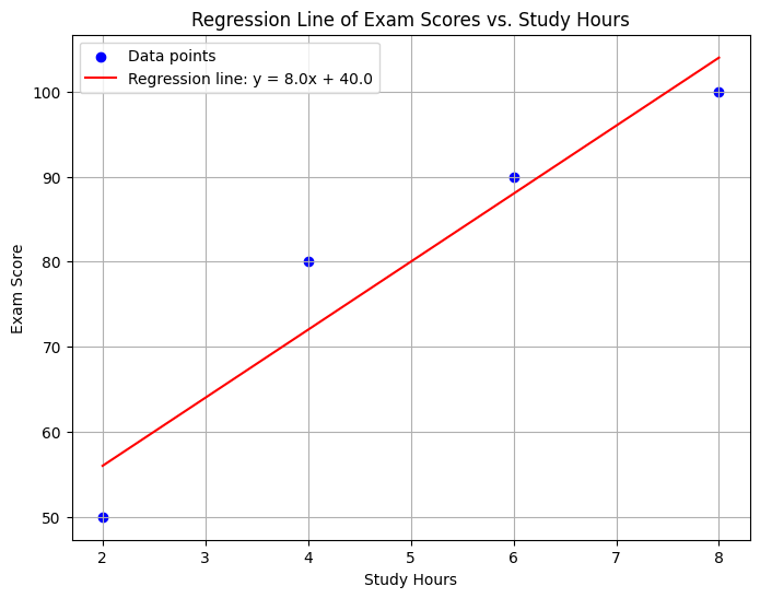
regression line = y = mx + b regression line = 8x + 40

code to plot the regression line in the graph

import numpy as np
import matplotlib.pyplot as plt

# Given data
study_hours = np.array([2, 4, 6, 8])
exam_scores = np.array([50, 80, 90, 100])
mean_x = 5
mean_y = 80

# Calculate the slope and intercept
sum_product_deviation_xy = 160
sum_square_deviation_x = 20

slope = sum_product_deviation_xy / sum_square_deviation_x
intercept = mean_y - slope * mean_x

# Regression line equation
x_line = np.linspace(min(study_hours), max(study_hours), 100)
y_line = slope * x_line + intercept

# Plot the data points and regression line
plt.figure(figsize=(8, 6))
plt.scatter(study_hours, exam_scores, color='blue', label='Data points')
plt.plot(x_line, y_line, color='red', label=f'Regression line: y = {slope:.1f}x + {intercept:.1f}')
plt.title('Regression Line of Exam Scores vs. Study Hours')
plt.xlabel('Study Hours')
plt.ylabel('Exam Score')
plt.legend()
plt.grid(True)
plt.show()

# Check if the solution provided matches calculated results
slope, intercept

lets get x and y points to plot the regression line

Study Hours	Exam Score
2	56
4	72
6	88
8	104

code to get x and y points for linear regression

# import libraries and recalculate
import numpy as np

# Data points
study_hours = np.array([2, 4, 6, 8])
exam_scores = np.array([50, 80, 90, 100])
mean_x = 5
mean_y = 80

# Calculations
sum_product_deviation_xy = 160
sum_square_deviation_x = 20

slope = sum_product_deviation_xy / sum_square_deviation_x
intercept = mean_y - slope * mean_x

# Get specific points for the regression line
x_points = study_hours
y_points = slope * x_points + intercept

# Display x and y points
list(zip(x_points, y_points))

Advantages of Linear Regression

• Simple to understand and interpret.
• Easy to implement.
• Can handle outliers and noise. (An outlier is a data point that is noticeably different from the rest.)

Disadvantages of Linear Regression

• Can be sensitive to outliers.
• Can be affected by multicollinearity (high correlation between independent variables).
• Can be less accurate for non-linear relationships.

Question: Predicting Price Based on Area Using Linear Regression

You are assigned with analyzing the relationship between the area of a property (in square meters) and its price (in thousands of USD). Below is the dataset:

Area (sq. m)	Price (*1000 USD)
8	10
10	13
12	16

Instructions:

1. Using linear regression, determine the relationship between the area and price.

   • Compute the slope and intercept of the regression line.
   • Derive the equation of the regression line in the form ( y = mx + b ), where (y) represents the price, and (x) represents the area.

2. Plot the data points and the regression line on a graph:

   • The (x)-axis should represent the area (sq. m).
   • The (y)-axis should represent the price (*1000 USD).

3. Use the regression equation to predict the price of a property with an area of 18 sq. m.

Deliverables:

• The regression equation.
• A graph displaying the data points and the regression line.
• The predicted price for an area of 18 sq. m.