Polynomial Regression

Polynomial Regression is an extension of linear regression that models the relationship between the independent variable (X) and the dependent variable (Y) as a polynomial. It is used when the relationship between (X) and (Y) is nonlinear and cannot be adequately captured by a straight line.

The general form of the polynomial regression equation is:

[ Y = b_0 + b_1X + b_2X^2 + b_3X^3 + ... + b_nX^n + ϵ(epsilon) ]

Where:

• (Y): Dependent variable
• (X, X^2, X^3, ..., X^n): Independent variables and their polynomial terms
• (b_0, b_1, b_2, ..., b_n): Coefficients
• ϵ(epsilon): Error term

---

When to Use Polynomial Regression?

1. The relationship between the dependent and independent variables is nonlinear.
2. Higher-order polynomials are needed to better fit the data.

---

Example: Modeling a Nonlinear Relationship

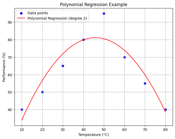
Suppose we have data showing the performance of a machine at different levels of temperature:

Temperature (°C)	Performance (%)
10	40
20	50
30	65
40	80
50	95
60	70
70	55
80	40

Clearly, the relationship is not linear. A polynomial regression can better model this behavior.

---

Code Example

Here’s how to perform polynomial regression and plot the results:

import numpy as np
import matplotlib.pyplot as plt
from sklearn.preprocessing import PolynomialFeatures
from sklearn.linear_model import LinearRegression

# Data
X = np.array([10, 20, 30, 40, 50, 60, 70, 80]).reshape(-1, 1)
Y = np.array([40, 50, 65, 80, 95, 70, 55, 40])

# Transform data to include polynomial features (degree 2)
poly = PolynomialFeatures(degree=2)
X_poly = poly.fit_transform(X)

# Fit polynomial regression model
model = LinearRegression()
model.fit(X_poly, Y)

# Generate predictions
X_range = np.linspace(10, 80, 100).reshape(-1, 1)
X_range_poly = poly.transform(X_range)
Y_pred = model.predict(X_range_poly)

# Plot
plt.figure(figsize=(8, 6))
plt.scatter(X, Y, color='blue', label='Data points')
plt.plot(X_range, Y_pred, color='red', label='Polynomial Regression (degree 2)')
plt.title('Polynomial Regression Example')
plt.xlabel('Temperature (°C)')
plt.ylabel('Performance (%)')
plt.legend()
plt.grid(True)
plt.show()

Advantages

1. Captures nonlinear relationships effectively.
2. Provides more flexibility than linear regression.

Limitations

1. Overfitting: High-degree polynomials may fit the training data well but fail to generalize.
2. Computational Complexity: Higher degrees can make computations more resource-intensive.