Logistic Regression

Logistic Regression is a statistical method used for binary classification problems. It predicts the probability that an observation belongs to one of two classes. Instead of fitting a straight line (as in linear regression), logistic regression uses the logit function (sigmoid curve) to model probabilities.

---

Logistic Regression Equation

The logistic regression model estimates the probability (p) of the dependent variable (Y) being 1, based on one or more independent variables (X):

$$p = \frac{1}{1 + e^{-(b_0 + b_1X_1 + b_2X_2)}}$$

Where:

• (p): Probability of (Y = 1)
• (b_0): Intercept
• (b_1, b_2, ldots, b_n): Coefficients for the independent variables
• (X_1, X_2, ldots, X_n): Independent variables
• (e): Euler's number (~2.718)

---

When to Use Logistic Regression?

1. Binary Classification: When the dependent variable has two possible outcomes (e.g., Yes/No, Pass/Fail, Spam/Not Spam).
2. Probability Estimation: When you need to predict the likelihood of an event occurring.

---

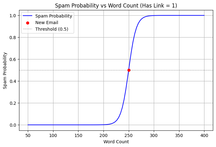
Example: Email Spam Classification

Suppose we have a dataset with features indicating email characteristics and whether the email is spam (1) or not (0):

Word Count (X_1)	Has Link (X_2)	Spam (Y)
50	0	0
300	1	1
200	0	0
400	1	1

Steps:

1. Fit the logistic regression model to the data.
2. Derive the coefficients (b_0), (b_1), and (b_2).
3. Use the equation: $$p = \frac{1}{1 + e^{-(b_0 + b_1X_1 + b_2X_2 + \ldots + b_nX_n)}}$$ to predict the probability of an email being spam.

---

Code Example

Here’s a simple implementation using Python:

# Re-importing necessary libraries and initializing the setup
import numpy as np
import pandas as pd
import matplotlib.pyplot as plt
from sklearn.linear_model import LogisticRegression

# Dataset
data = {
    "Word Count": [50, 300, 200, 400],
    "Has Link": [0, 1, 0, 1],
    "Spam": [0, 1, 0, 1]
}

df = pd.DataFrame(data)

# Features and target variable
X = df[["Word Count", "Has Link"]]
y = df["Spam"]

# Train logistic regression model
model = LogisticRegression()
model.fit(X, y)

# Predict probability for a new email
new_email = np.array([[250, 1]])  # Word Count = 250, Has Link = 1
spam_probability = model.predict_proba(new_email)[0][1]

# Define the range for Word Count and Has Link
word_count_range = np.linspace(50, 400, 100)
has_link = 1  # Considering emails with links

# Calculate spam probabilities for different word counts
probabilities = [
    model.predict_proba([[wc, has_link]])[0][1] for wc in word_count_range
]

# Plot
plt.figure(figsize=(8, 5))
plt.plot(word_count_range, probabilities, label="Spam Probability", color="blue")
plt.scatter(new_email[0][0], spam_probability, color="red", label="New Email", zorder=5)
plt.title("Spam Probability vs Word Count (Has Link = 1)")
plt.xlabel("Word Count")
plt.ylabel("Spam Probability")
plt.axhline(0.5, color='gray', linestyle='--', linewidth=0.7, label="Threshold (0.5)")
plt.legend()
plt.grid(True)
plt.show()

Advantages

1. Simple to implement and interpret.
2. Efficient for binary classification problems.
3. Provides probabilistic predictions.

Limitations

1. Assumes a linear relationship between predictors and the log-odds.
2. Sensitive to multicollinearity among predictors.
3. Limited to binary classification (though extensions like multinomial logistic regression exist for multiple classes).