Enhancement

To enhance your linear regression, consider incorporating the following topics:

Bias

• Definition: Bias refers to the error introduced by approximating a real-world problem, which may be complex, using a simplified model.
• Effect: High bias leads to underfitting, where the model is too simple to capture the underlying patterns in the data.

---

Variance

• Definition: Variance refers to the error introduced due to the model's sensitivity to small fluctuations in the training data.
• Effect: High variance leads to overfitting, where the model captures noise in the training data as if it were a pattern.

---

Bias-Variance Trade-off

• Goal: Find the optimal balance between bias and variance to minimize the total error.
• Total error can be expressed as:

$$\text{Total Error} = \text{Bias}^2 + \text{Variance} + \text{Irreducible Error}$$

• Irreducible Error: Noise inherent in the data that no model can explain.

---

Graphical Representation

1. Bias vs. Variance

A graph of model complexity on the x-axis and error on the y-axis illustrates:

• High Bias (Underfitting): On the left, where the model is too simple.
• High Variance (Overfitting): On the right, where the model is too complex.
• Optimal Point: Somewhere in the middle, where the total error is minimized.

---

Example Graph

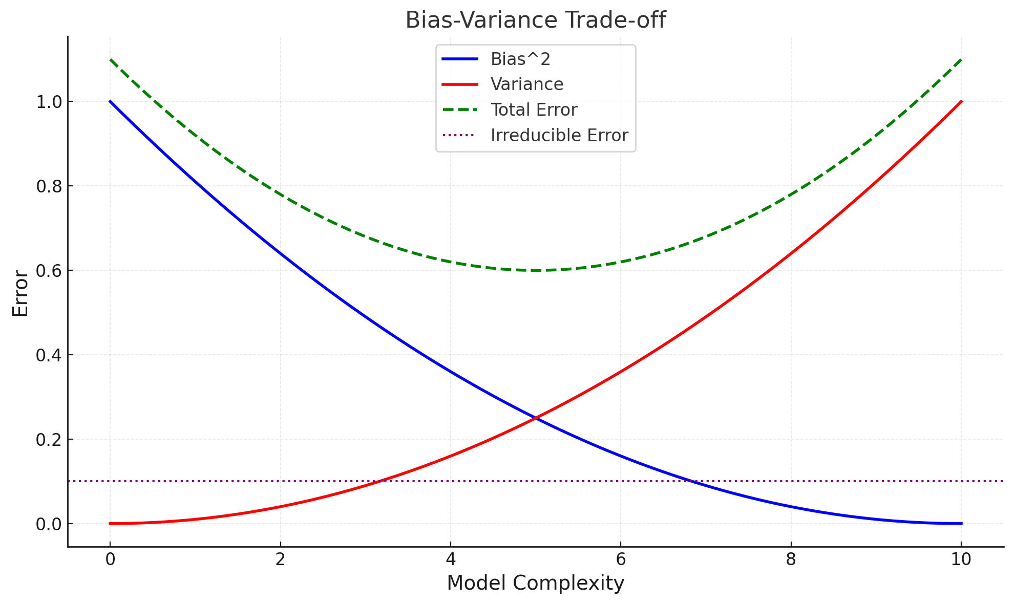
Here is the graph illustrating the Bias-Variance Trade-off:

1. Bias² (Blue Curve): Decreases as model complexity increases, indicating that more complex models better fit the data.
2. Variance (Red Curve): Increases with model complexity, showing that overly complex models are sensitive to data fluctuations.
3. Total Error (Green Dashed Curve): The sum of bias², variance, and irreducible error. It shows the optimal point of model complexity where the error is minimized.
4. Irreducible Error (Purple Dotted Line): Represents the noise in the data that cannot be reduced by any model.

This graph visually demonstrates the need to balance bias and variance for optimal model performance.

2. Summarizing

Here’s a table summarizing the relationship between bias, variance, underfitting, and overfitting:

Condition	Bias	Variance	Description	Model Behavior
High Bias, Low Variance	High (simplistic assumptions)	Low (not sensitive to data fluctuations)	Model is too simple to capture the data's patterns.	Underfitting
Low Bias, High Variance	Low (complex model captures data patterns)	High (sensitive to data noise)	Model fits the training data too closely, including noise.	Overfitting
Low Bias, Low Variance	Low (accurately models patterns)	Low (generalizes well to unseen data)	Ideal model that balances bias and variance.	Good Fit
High Bias, High Variance	High (poor model assumptions)	High (erratic and sensitive)	Rare but indicates both underfitting and overfitting issues.	Poor Performance

---

Key Points:

• High Bias → Underfitting: The model is too rigid and misses the true patterns.
• High Variance → Overfitting: The model is too flexible and captures noise as patterns.
• Low Bias, Low Variance → Good Fit: Achieved with an optimal balance.

Good Fit, Overfitting, and Underfitting

These terms describe how well a machine learning model captures the underlying patterns in the data. Let’s explore them:

---

1. Underfitting

• Definition: Occurs when a model is too simple to capture the underlying structure of the data.
• Characteristics:
  • High bias and low variance.
  • Poor performance on both training and testing data.
• Example: A linear model trying to fit a non-linear dataset.
• Solution:
  • Increase model complexity.
  • Use additional or better features.
  • Reduce regularization.

---

2. Overfitting

• Definition: Occurs when a model is too complex and captures noise or random fluctuations in the training data.
• Characteristics:
  • Low bias and high variance.
  • Excellent performance on training data but poor generalization to testing data.
• Example: A high-degree polynomial model fitting noise in the data.
• Solution:
  • Reduce model complexity.
  • Use regularization techniques (e.g., L1/L2 regularization).
  • Increase the size of the training dataset.

---

3. Good Fit

• Definition: A model that captures the underlying patterns in the data without overfitting or underfitting.
• Characteristics:
  • Balanced bias and variance.
  • Good performance on both training and testing data.
• Example: A model with just the right level of complexity for the given data.
• Solution: Achieved through proper model selection, hyperparameter tuning, and validation.

---

Graphical Representation

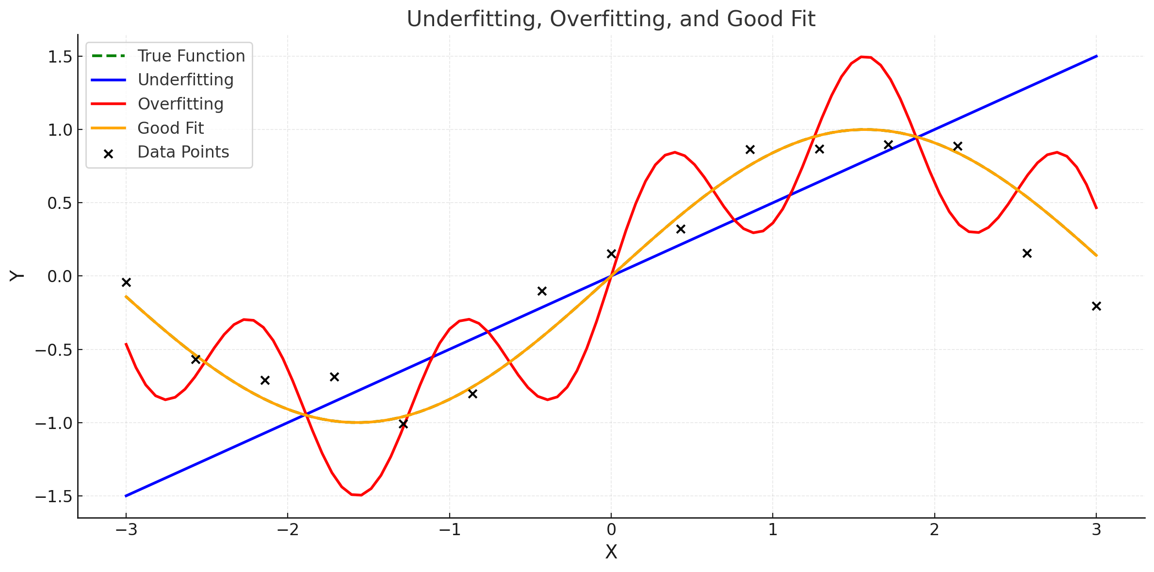
Here is the graph illustrating Underfitting, Overfitting, and Good Fit:

1. True Function (Green Dashed Line): Represents the actual underlying pattern in the data (e.g., ( \sin(x) )).
2. Underfitting (Blue Line): The model is too simple (e.g., a linear fit) and fails to capture the pattern in the data.
3. Overfitting (Red Line): The model is too complex, fitting the noise in the data rather than the true pattern.
4. Good Fit (Orange Line): The model captures the underlying pattern without fitting the noise, achieving a balance between bias and variance.
5. Data Points (Black Dots): Represent the observed data, which contains some noise.

This visualization helps distinguish the behavior of models with varying levels of complexity.

---

Hyperparameters:

Definition: Hyperparameters are external configurations set before training a model, which govern the training process and model architecture. They are not learned from the data.

Usage: Selecting appropriate hyperparameters is crucial for model performance. Techniques like cross-validation can help in tuning hyperparameters to achieve a balance between bias and variance, thus avoiding overfitting and underfitting.

They define the training process and model structure but are not updated or learned during training. Common hyperparameters include learning rate, batch size, number of epochs, and regularization strength.

1. Learning Rate: Controls the step size for updating model weights during training.

   • Small: Slower training, but more precise.
   • Large: Faster training, but risk of overshooting the optimal point.

2. Batch Size: The number of training samples processed before updating model weights.

   • Small: More updates, higher variance, slower training.
   • Large: Fewer updates, faster but less generalized.

3. Number of Epochs: How many times the entire dataset is passed through the model during training.

   • Few Epochs: May underfit.
   • Too Many Epochs: May overfit.

4. Regularization Strength: A penalty term to prevent overfitting by discouraging overly complex models.

   • High Strength: Simpler models, less overfitting.
   • Low Strength: More complex models, risk of overfitting.

Characteristics of Hyperparameters:

1. Set by the User: You manually define them before training the model.
2. External to Training: Unlike parameters (like weights(Coefficients) and biases(Intercept) in linear regression), hyperparameters are not learned or optimized from the training data.
3. Control the Model's Behavior: They affect how the model learns from the data, its complexity, and its performance.

Examples of Hyperparameters:

• Learning Rate: Determines the step size during optimization.
• Number of Epochs: Specifies how many times the model will pass through the entire training dataset.
• Batch Size: Defines the number of samples processed before updating the model.
• Regularization Parameters: Help avoid overfitting (e.g., L1 or L2 regularization coefficients).
• Model Architecture Choices: Such as the number of layers or neurons in a neural network.

Why Hyperparameters Are Not Learned:

Hyperparameters govern how the learning process is conducted, and their values are chosen before training starts. If they were learned from the data, it would introduce complexity and often instability in the training process.

However, there are automated techniques (like grid search, random search, or Bayesian optimization) to systematically select hyperparameters, making them less of a trial-and-error process.